1. NN模型如下

神經(jīng)網(wǎng)絡(luò)整體架構(gòu)內(nèi)容可參考之前的云筆記《06_神經(jīng)網(wǎng)絡(luò)整體架構(gòu)》

http://note.youdao.com/noteshare?id=2c27bbf6625d75e4173d9fcbeea5e8c1&sub=7F4BC70112524F9289531EC6AE435E14

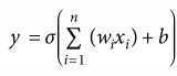
其中，

n是指的樣本數(shù)

Mnist數(shù)據(jù)集 784是28×28×1 灰度圖 channel = 1

wb是指的權(quán)重參數(shù)

輸出的是10分類的得分值，也可以接softmax分類器

out是L2層和輸出層之間的關(guān)系

256 128 10是指的神經(jīng)元數(shù)量

2. 構(gòu)造參數(shù)

函數(shù)構(gòu)造

3. Code

1. 網(wǎng)絡(luò)模型架構(gòu)搭建

導(dǎo)入相應(yīng)數(shù)據(jù)

import numpy as npimport tensorflow as tfimport matplotlib.pyplot as pltimport input_datamnist = input_data.read_data_sets('data/', one_hot=True)network topologies

# 網(wǎng)絡(luò)拓?fù)?network topologies# layer中神經(jīng)元數(shù)量n_hidden_1 =256n_hidden_2 =128# 輸入數(shù)據(jù)的像素點(diǎn) 28x28x1n_input =784# 10分類n_classes =10input and output

x = tf.placeholder("float",[None,n_input])y = tf.placeholder("float",[None,n_classes])network parameters

# network parameters# 方差stddev =0.1# random_normal 高斯初始化weights ={'w1': tf.Variable(tf.random_normal([n_input,n_hidden_1],stddev=stddev)),'w2': tf.Variable(tf.random_normal([n_hidden_1,n_hidden_2],stddev=stddev)),'out': tf.Variable(tf.random_normal([n_hidden_2,n_classes],stddev=stddev))}# 對(duì)于 b 零值初始化也可以biases ={'b1': tf.Variable(tf.random_normal([n_hidden_1])),'b2': tf.Variable(tf.random_normal([n_hidden_2])),'out': tf.Variable(tf.random_normal([n_classes]))}print("Network Ready")output

NetworkReady可以看到網(wǎng)絡(luò)模型架構(gòu)搭建成功

2.訓(xùn)練網(wǎng)絡(luò)模型

定義前向傳播函數(shù)

# 定義前向傳播函數(shù)def multilayer_perceptron(_X, _weights, _biases):# 之所以加 sigmoid 是因?yàn)槊恳粋€(gè) hidden layer 都有一個(gè)非線性函數(shù)layer_1 = tf.nn.sigmoid(tf.add(tf.matmul(_X, _weights['w1']), _biases['b1']))layer_2 = tf.nn.sigmoid(tf.add(tf.matmul(layer_1, _weights['w2']), _biases['b2']))return(tf.matmul(layer_2, _weights['out'])+ _biases['out'])反向傳播

（1）將前向傳播預(yù)測(cè)值

# predictionpred = multilayer_perceptron(x, weights, biases)（2）定義損失函數(shù)

# 首先定義損失函數(shù) softmax_cross_entropy_with_logits 交叉熵函數(shù)# 交叉熵函數(shù)的輸入有 pred : 網(wǎng)絡(luò)的預(yù)測(cè)值 （前向傳播的結(jié)果）# y : 實(shí)際的label值# 將兩參數(shù)的一系列的比較結(jié)果，除以 batch 求平均之后的 loss 返回給 cost 損失值cost = tf.reduce_mean(tf.nn.softmax_cross_entropy_with_logits(pred, y))（3）梯度下降最優(yōu)化

optm = tf.train.GradientDescentOptimizer(learning_rate =0.001).minimize(cost)（4）精確值

具體解釋詳見(jiàn)上一篇筆記《06_迭代完成邏輯回歸模型》

corr = tf.equal(tf.argmax(pred,1), tf.argmax(y,1))accr = tf.reduce_mean(tf.cast(corr,"float"))（5）初始化

# initializerinit = tf.global_variables_initializer()print("Function ready")output

Function ready可以看出傳播中的參數(shù)和優(yōu)化模型搭建成功

3. Train and Test

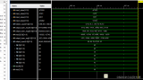
training_epochs =20# 每次 iteration 的樣本batch_size =100# 每四個(gè) epoch 打印一次結(jié)果display_step =4# lanch the graphsess = tf.Session()sess.run(init)# optimizefor epoch in range(training_epochs):# 初始，平均 loss = 0avg_cost =0total_batch =int(mnist.train.num_examples/batch_size)# iterationfor i in range(total_batch):# 通過(guò) next_batch 返回相應(yīng)的 batch_xs，batch_ysbatch_xs, batch_ys = mnist.train.next_batch(batch_size)feeds ={x: batch_xs, y: batch_ys}sess.run(optm, feed_dict = feeds)avg_cost += sess.run(cost, feed_dict = feeds)avg_cost = avg_cost / total_batch# displayif(epoch+1)% display_step ==0:print("Epoch: %03d/%03d cost: %.9f "%(epoch, training_epochs, avg_cost))feeds ={x: batch_xs, y: batch_ys}train_acc = sess.run(accr, feed_dict = feeds)print("train accuracy: %.3f"%(train_acc))feeds ={x: mnist.test.images, y: mnist.test.labels}test_acc = sess.run(accr, feed_dict = feeds)print("test accuracy: %.3f"%(test_acc))print("optimization finished")output

Epoch:003/020 cost:2.273774184train accuracy:0.250test accuracy:0.197Epoch:007/020 cost:2.240329206train accuracy:0.270test accuracy:0.311Epoch:011/020 cost:2.203503076train accuracy:0.370test accuracy:0.404Epoch:015/020 cost:2.161286944train accuracy:0.490test accuracy:0.492Epoch:019/020 cost:2.111541148train accuracy:0.410test accuracy:0.534optimization finished20個(gè)batch每個(gè)batch 100個(gè)樣本，每隔4個(gè)batch打印一次

處理器：Intel Core i5-6200U CPU @ 2.30GHz 2.04GHz

04 epoch：train+test, cost_time: 25’40”

08 epoch：train+test, cost_time: 50’29”

12 epoch：train+test, cost_time: 74’42”

16 epoch：train+test, cost_time: 98’63”

20 epoch：train+test, cost_time: 121’49”