“PyTorch 深度學(xué)習(xí):60分鐘快速入門”為 PyTorch 官網(wǎng)教程，網(wǎng)上已經(jīng)有部分翻譯作品，隨著PyTorch1.0 版本的公布，這個(gè)教程有較大的代碼改動(dòng)，本人對(duì)教程進(jìn)行重新翻譯，并測(cè)試運(yùn)行了官方代碼，制作成 Jupyter Notebook文件（中文注釋）在 github 予以公布。

本教程的目標(biāo)：

在高層次上理解PyTorch的張量(Tensor)庫(kù)和神經(jīng)網(wǎng)絡(luò)

訓(xùn)練一個(gè)小型神經(jīng)網(wǎng)絡(luò)對(duì)圖像進(jìn)行分類

本教程假設(shè)您對(duì)numpy有基本的了解

注意： 務(wù)必確認(rèn)您已經(jīng)安裝了 torch 和 torchvision 兩個(gè)包。

目錄

一、Pytorch是什么？

二、AUTOGRAD

三、神經(jīng)網(wǎng)絡(luò)

四、訓(xùn)練一個(gè)分類器

五、數(shù)據(jù)并行

一、PyTorch 是什么

他是一個(gè)基于Python的科學(xué)計(jì)算包，目標(biāo)用戶有兩類

為了使用GPU來(lái)替代numpy

一個(gè)深度學(xué)習(xí)研究平臺(tái)：提供最大的靈活性和速度

開始

張量（Tensors)

張量類似于numpy的ndarrays，不同之處在于張量可以使用GPU來(lái)加快計(jì)算。

from __future__ import print_functionimport torch

構(gòu)建一個(gè)未初始化的5*3的矩陣：

x = torch.Tensor(5, 3)print(x)

輸出 ：

tensor([[ 0.0000e+00, 0.0000e+00, 1.3004e-42], [ 0.0000e+00, 7.0065e-45, 0.0000e+00], [-3.8593e+35, 7.8753e-43, 0.0000e+00], [ 0.0000e+00, 1.8368e-40, 0.0000e+00], [-3.8197e+35, 7.8753e-43, 0.0000e+00]])

構(gòu)建一個(gè)零矩陣，使用long的類型

x = torch.zeros(5, 3, dtype=torch.long)print(x)

輸出：

tensor([[0, 0, 0], [0, 0, 0], [0, 0, 0], [0, 0, 0], [0, 0, 0]])

從數(shù)據(jù)中直接構(gòu)建一個(gè)張量(tensor)：

x = torch.tensor([5.5, 3])print(x)

輸出:

tensor([5.5000, 3.0000])

或者在已有的張量(tensor)中構(gòu)建一個(gè)張量(tensor). 這些方法將重用輸入張量(tensor)的屬性，例如， dtype，除非用戶提供新值

x = x.new_ones(5, 3, dtype=torch.double) # new_* methods take in sizesprint(x)x = torch.randn_like(x, dtype=torch.float) # 覆蓋類型!print(x) # result 的size相同

輸出：

tensor([[1., 1., 1.], [1., 1., 1.], [1., 1., 1.], [1., 1., 1.], [1., 1., 1.]], dtype=torch.float64)tensor([[ 1.1701, -0.8342, -0.6769], [-1.3060, 0.3636, 0.6758], [ 1.9133, 0.3494, 1.1412], [ 0.9735, -0.9492, -0.3082], [ 0.9469, -0.6815, -1.3808]])

獲取張量(tensor)的大小

print(x.size())

輸出：

torch.Size([5, 3])

注意

torch.Size實(shí)際上是一個(gè)元組，所以它支持元組的所有操作。

操作

張量上的操作有多重語(yǔ)法形式，下面我們以加法為例進(jìn)行講解。

語(yǔ)法1

y = torch.rand(5, 3)print(x + y)

輸出:

tensor([[ 1.7199, -0.1819, -0.1543], [-0.5413, 1.1591, 1.4098], [ 2.0421, 0.5578, 2.0645], [ 1.7301, -0.3236, 0.4616], [ 1.2805, -0.4026, -0.6916]])

語(yǔ)法二

print(torch.add(x, y))

輸出:

tensor([[ 1.7199, -0.1819, -0.1543], [-0.5413, 1.1591, 1.4098], [ 2.0421, 0.5578, 2.0645], [ 1.7301, -0.3236, 0.4616], [ 1.2805, -0.4026, -0.6916]])

語(yǔ)法三：給出一個(gè)輸出張量作為參數(shù)

result = torch.empty(5, 3)torch.add(x, y, out=result)print(result)

輸出:

tensor([[ 1.7199, -0.1819, -0.1543], [-0.5413, 1.1591, 1.4098], [ 2.0421, 0.5578, 2.0645], [ 1.7301, -0.3236, 0.4616], [ 1.2805, -0.4026, -0.6916]])

語(yǔ)法四：原地操作（in-place）

# 把x加到y(tǒng)上y.add_(x)print(y)

輸出:

tensor([[ 1.7199, -0.1819, -0.1543], [-0.5413, 1.1591, 1.4098], [ 2.0421, 0.5578, 2.0645], [ 1.7301, -0.3236, 0.4616], [ 1.2805, -0.4026, -0.6916]])

注意

任何在原地(in-place)改變張量的操作都有一個(gè)’_‘后綴。例如x.copy_(y), x.t_()操作將改變x.

你可以使用所有的numpy索引操作。你可以使用各種類似標(biāo)準(zhǔn)NumPy的花哨的索引功能

print(x[:, 1])

輸出：

tensor([-0.8342, 0.3636, 0.3494, -0.9492, -0.6815])

調(diào)整大小：如果要調(diào)整張量/重塑張量，可以使用torch.view：

x = torch.randn(4, 4)y = x.view(16)z = x.view(-1, 8) # -1的意思是沒(méi)有指定維度print(x.size(), y.size(), z.size())

輸出：

torch.Size([4, 4]) torch.Size([16]) torch.Size([2, 8])

如果你有一個(gè)單元素張量，使用.item()將值作為Python數(shù)字

x = torch.randn(1)print(x)print(x.item())

輸出：

tensor([0.3441])0.34412217140197754

numpy 橋

把一個(gè) torch 張量轉(zhuǎn)換為 numpy 數(shù)組或者反過(guò)來(lái)都是很簡(jiǎn)單的。

Torch 張量和 numpy 數(shù)組將共享潛在的內(nèi)存，改變其中一個(gè)也將改變另一個(gè)。

把 Torch 張量轉(zhuǎn)換為 numpy 數(shù)組

a = torch.ones(5)print(a)

輸出：

tensor([1., 1., 1., 1., 1.])

輸入：

b = a.numpy()print(b)print(type(b))

輸出：

[ 1. 1. 1. 1. 1.]

通過(guò)如下操作，我們看一下numpy數(shù)組的值如何在改變。

a.add_(1)print(a)print(b)

輸出：

tensor([2., 2., 2., 2., 2.])[ 2. 2. 2. 2. 2.]

把 numpy 數(shù)組轉(zhuǎn)換為 torch 張量

看看改變 numpy 數(shù)組如何自動(dòng)改變 torch 張量。

import numpy as npa = np.ones(5)b = torch.from_numpy(a)np.add(a, 1, out=a)print(a)print(b)

輸出：

[ 2. 2. 2. 2. 2.]tensor([2., 2., 2., 2., 2.], dtype=torch.float64)

所有在CPU上的張量，除了字符張量，都支持在numpy之間轉(zhuǎn)換。

CUDA 張量

可以使用.to方法將張量移動(dòng)到任何設(shè)備上。

# let us run this cell only if CUDA is available# We will use ``torch.device`` objects to move tensors in and out of GPUif torch.cuda.is_available(): device = torch.device("cuda") # a CUDA device object y = torch.ones_like(x, device=device) # directly create a tensor on GPU x = x.to(device) # or just use strings ``.to("cuda")`` z = x + y print(z) print(z.to("cpu", torch.double)) # ``.to`` can also change dtype together!

腳本總運(yùn)行時(shí)間:0.003秒

二、Autograd: 自動(dòng)求導(dǎo)(automatic differentiation)

PyTorch 中所有神經(jīng)網(wǎng)絡(luò)的核心是autograd包.我們首先簡(jiǎn)單介紹一下這個(gè)包,然后訓(xùn)練我們的第一個(gè)神經(jīng)網(wǎng)絡(luò).

autograd包為張量上的所有操作提供了自動(dòng)求導(dǎo).它是一個(gè)運(yùn)行時(shí)定義的框架,這意味著反向傳播是根據(jù)你的代碼如何運(yùn)行來(lái)定義,并且每次迭代可以不同.

接下來(lái)我們用一些簡(jiǎn)單的示例來(lái)看這個(gè)包:

張量(Tensor)

torch.Tensor是包的核心類。如果將其屬性.requires_grad設(shè)置為True，則會(huì)開始跟蹤其上的所有操作。完成計(jì)算后，您可以調(diào)用.backward()并自動(dòng)計(jì)算所有梯度。此張量的梯度將累積到.grad屬性中。

要阻止張量跟蹤歷史記錄，可以調(diào)用.detach()將其從計(jì)算歷史記錄中分離出來(lái)，并防止將來(lái)的計(jì)算被跟蹤。

要防止跟蹤歷史記錄（和使用內(nèi)存），您還可以使用torch.no_grad()包裝代碼塊：在評(píng)估模型時(shí)，這可能特別有用，因?yàn)槟Ｐ涂赡芫哂衦equires_grad = True的可訓(xùn)練參數(shù)，但我們不需要梯度。

還有一個(gè)類對(duì)于autograd實(shí)現(xiàn)非常重要 - Function。

Tensor和Function互相連接并構(gòu)建一個(gè)非循環(huán)圖構(gòu)建一個(gè)完整的計(jì)算過(guò)程。每個(gè)張量都有一個(gè).grad_fn屬性，該屬性引用已創(chuàng)建Tensor的Function（除了用戶創(chuàng)建的Tensors - 它們的grad_fn為None）。

如果要計(jì)算導(dǎo)數(shù)，可以在Tensor上調(diào)用.backward()。如果Tensor是標(biāo)量（即它包含一個(gè)元素?cái)?shù)據(jù)），則不需要為backward()指定任何參數(shù)，但是如果它有更多元素，則需要指定一個(gè)梯度參數(shù)，該參數(shù)是匹配形狀的張量。

import torch

創(chuàng)建一個(gè)張量并設(shè)置requires_grad = True以跟蹤它的計(jì)算

x = torch.ones(2, 2, requires_grad=True)print(x)

輸出:

tensor([[1., 1.], [1., 1.]], requires_grad=True)

在張量上執(zhí)行操作:

y = x + 2print(y)

輸出:

tensor([[3., 3.], [3., 3.]], grad_fn=)

因?yàn)閥是通過(guò)一個(gè)操作創(chuàng)建的,所以它有g(shù)rad_fn,而x是由用戶創(chuàng)建,所以它的grad_fn為None.

print(y.grad_fn)print(x.grad_fn)

輸出:

None

在y上執(zhí)行操作

z = y * y * 3out = z.mean()print(z, out)

輸出:

tensor([[27., 27.], [27., 27.]], grad_fn=) tensor(27., grad_fn=)

.requires_grad_(...)就地更改現(xiàn)有的Tensor的requires_grad標(biāo)志。 如果沒(méi)有給出，輸入標(biāo)志默認(rèn)為False。

a = torch.randn(2, 2)a = ((a * 3) / (a - 1))print(a.requires_grad)a.requires_grad_(True)print(a.requires_grad)b = (a * a).sum()print(b.grad_fn)

輸出：

FalseTrue

梯度(Gradients)

現(xiàn)在我們來(lái)執(zhí)行反向傳播,out.backward()相當(dāng)于執(zhí)行out.backward(torch.tensor(1.))

out.backward()

輸出out對(duì)x的梯度d(out)/dx:

print(x.grad)

輸出:

tensor([[4.5000, 4.5000], [4.5000, 4.5000]])

你應(yīng)該得到一個(gè)值全為4.5的矩陣,我們把張量out稱為"o". 則：

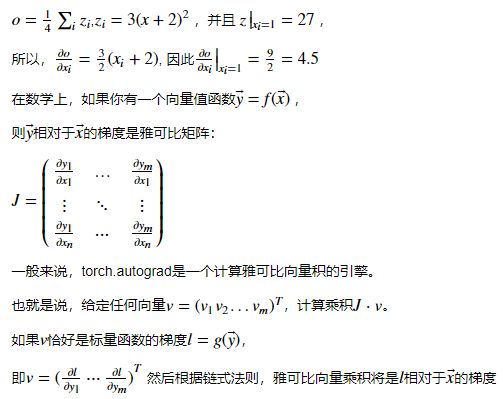
雅可比向量積的這種特性使得將外部梯度饋送到具有非標(biāo)量輸出的模型中非常方便。

現(xiàn)在讓我們來(lái)看一個(gè)雅可比向量積的例子：

x = torch.randn(3, requires_grad=True)y = x * 2while y.data.norm() < 1000: ? ?y = y * 2print(y)

輸出：

tensor([ 384.5854, -13.6405, -1049.2870], grad_fn=)

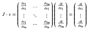
現(xiàn)在在這種情況下，y不再是標(biāo)量。torch.autograd無(wú)法直接計(jì)算完整雅可比行列式，但如果我們只想要雅可比向量積，只需將向量作為參數(shù)向后傳遞：

v = torch.tensor([0.1, 1.0, 0.0001], dtype=torch.float)y.backward(v)print(x.grad)

輸出：

tensor([5.1200e+01, 5.1200e+02, 5.1200e-02])

您還可以通過(guò)torch.no_grad()代碼，在張量上使用.requires_grad = True來(lái)停止使用跟蹤歷史記錄。

print(x.requires_grad)print((x ** 2).requires_grad)with torch.no_grad(): print((x ** 2).requires_grad)

輸出：

TrueTrueFalse

關(guān)于 autograd 和 Function 的文檔在 http://pytorch.org/docs/autograd

三、神經(jīng)網(wǎng)絡(luò)

可以使用torch.nn包來(lái)構(gòu)建神經(jīng)網(wǎng)絡(luò).

你已知道autograd包，nn包依賴autograd包來(lái)定義模型并求導(dǎo).一個(gè)nn.Module包含各個(gè)層和一個(gè)forward(input)方法,該方法返回output.

例如,我們來(lái)看一下下面這個(gè)分類數(shù)字圖像的網(wǎng)絡(luò).

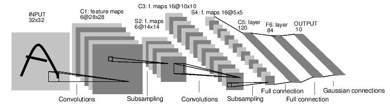
convnet

他是一個(gè)簡(jiǎn)單的前饋神經(jīng)網(wǎng)絡(luò),它接受一個(gè)輸入,然后一層接著一層的輸入,直到最后得到結(jié)果.

神經(jīng)網(wǎng)絡(luò)的典型訓(xùn)練過(guò)程如下:

定義神經(jīng)網(wǎng)絡(luò)模型,它有一些可學(xué)習(xí)的參數(shù)(或者權(quán)重);

在數(shù)據(jù)集上迭代;

通過(guò)神經(jīng)網(wǎng)絡(luò)處理輸入;

計(jì)算損失(輸出結(jié)果和正確值的差距大小)

將梯度反向傳播會(huì)網(wǎng)絡(luò)的參數(shù);

更新網(wǎng)絡(luò)的參數(shù),主要使用如下簡(jiǎn)單的更新原則:

weight = weight - learning_rate * gradient

定義網(wǎng)絡(luò)

我們先定義一個(gè)網(wǎng)絡(luò)

import torchimport torch.nn as nnimport torch.nn.functional as Fclass Net(nn.Module): def __init__(self): super(Net, self).__init__() # 1 input image channel, 6 output channels, 5x5 square convolution # kernel self.conv1 = nn.Conv2d(1, 6, 5) self.conv2 = nn.Conv2d(6, 16, 5) # an affine operation: y = Wx + b self.fc1 = nn.Linear(16 * 5 * 5, 120) self.fc2 = nn.Linear(120, 84) self.fc3 = nn.Linear(84, 10) def forward(self, x): # Max pooling over a (2, 2) window x = F.max_pool2d(F.relu(self.conv1(x)), (2, 2)) # If the size is a square you can only specify a single number x = F.max_pool2d(F.relu(self.conv2(x)), 2) x = x.view(-1, self.num_flat_features(x)) x = F.relu(self.fc1(x)) x = F.relu(self.fc2(x)) x = self.fc3(x) return x def num_flat_features(self, x): size = x.size()[1:] # all dimensions except the batch dimension num_features = 1 for s in size: num_features *= s return num_featuresnet = Net()print(net)

輸出:

Net( (conv1): Conv2d(1, 6, kernel_size=(5, 5), stride=(1, 1)) (conv2): Conv2d(6, 16, kernel_size=(5, 5), stride=(1, 1)) (fc1): Linear(in_features=400, out_features=120, bias=True) (fc2): Linear(in_features=120, out_features=84, bias=True) (fc3): Linear(in_features=84, out_features=10, bias=True))

你只需定義forward函數(shù),backward函數(shù)(計(jì)算梯度)在使用autograd時(shí)自動(dòng)為你創(chuàng)建.你可以在forward函數(shù)中使用Tensor的任何操作.

net.parameters()返回模型需要學(xué)習(xí)的參數(shù)。

params = list(net.parameters())print(len(params))print(params[0].size())

輸出:

10torch.Size([6, 1, 5, 5])f

讓我們嘗試一個(gè)隨機(jī)的 32x32 輸入。 注意：此網(wǎng)絡(luò)（LeNet）的預(yù)期輸入大小為 32x32。 要在MNIST數(shù)據(jù)集上使用此網(wǎng)絡(luò)，請(qǐng)將數(shù)據(jù)集中的圖像大小調(diào)整為 32x32。

input = torch.randn(1, 1, 32, 32)out = net(input)print(out)

輸出:

tensor([[-0.1217, 0.0449, -0.0392, -0.1103, -0.0534, -0.1108, -0.0565, 0.0116, 0.0867, 0.0102]], grad_fn=)

將所有參數(shù)的梯度緩存清零,然后進(jìn)行隨機(jī)梯度的的反向傳播.

net.zero_grad()out.backward(torch.randn(1, 10))

注意

torch.nn只支持小批量輸入,整個(gè)torch.nn包都只支持小批量樣本,而不支持單個(gè)樣本

??例如,nn.Conv2d將接受一個(gè)4維的張量,每一維分別是：

nSamples×nChannels×Height×Width(樣本數(shù)*通道數(shù)*高*寬).??

如果你有單個(gè)樣本,只需使用input.unsqueeze(0)來(lái)添加其它的維數(shù).

在繼續(xù)之前,我們回顧一下到目前為止見過(guò)的所有類.

回顧

torch.Tensor-支持自動(dòng)編程操作（如backward()）的多維數(shù)組。 同時(shí)保持梯度的張量。

nn.Module-神經(jīng)網(wǎng)絡(luò)模塊.封裝參數(shù),移動(dòng)到GPU上運(yùn)行,導(dǎo)出,加載等

nn.Parameter-一種張量,當(dāng)把它賦值給一個(gè)Module時(shí),被自動(dòng)的注冊(cè)為參數(shù).

autograd.Function-實(shí)現(xiàn)一個(gè)自動(dòng)求導(dǎo)操作的前向和反向定義, 每個(gè)張量操作都會(huì)創(chuàng)建至少一個(gè)Function節(jié)點(diǎn)，該節(jié)點(diǎn)連接到創(chuàng)建張量并對(duì)其歷史進(jìn)行編碼的函數(shù)。

損失函數(shù)

一個(gè)損失函數(shù)接受一對(duì)(output, target)作為輸入(output為網(wǎng)絡(luò)的輸出,target為實(shí)際值),計(jì)算一個(gè)值來(lái)估計(jì)網(wǎng)絡(luò)的輸出和目標(biāo)值相差多少.

在nn包中有幾種不同的損失函數(shù).一個(gè)簡(jiǎn)單的損失函數(shù)是:nn.MSELoss,他計(jì)算輸入(個(gè)人認(rèn)為是網(wǎng)絡(luò)的輸出)和目標(biāo)值之間的均方誤差.

例如:

output = net(input)target = torch.randn(10) # a dummy target, for exampletarget = target.view(1, -1) # make it the same shape as outputcriterion = nn.MSELoss()loss = criterion(output, target)print(loss)

輸出:

tensor(0.5663, grad_fn=)

現(xiàn)在,你反向跟蹤loss,使用它的.grad_fn屬性,你會(huì)看到向下面這樣的一個(gè)計(jì)算圖:

input -> conv2d -> relu -> maxpool2d -> conv2d -> relu -> maxpool2d -> view -> linear -> relu -> linear -> relu -> linear -> MSELoss -> loss

所以, 當(dāng)你調(diào)用loss.backward(),整個(gè)圖被區(qū)分為損失以及圖中所有具有requires_grad = True的張量，并且其.grad張量的梯度累積。

為了說(shuō)明,我們反向跟蹤幾步:

print(loss.grad_fn) # MSELossprint(loss.grad_fn.next_functions[0][0]) # Linearprint(loss.grad_fn.next_functions[0][0].next_functions[0][0])

輸出:

反向傳播

為了反向傳播誤差,我們所需做的是調(diào)用loss.backward().你需要清除已存在的梯度,否則梯度將被累加到已存在的梯度。

現(xiàn)在,我們將調(diào)用loss.backward(),并查看conv1層的偏置項(xiàng)在反向傳播前后的梯度。

net.zero_grad() # zeroes the gradient buffers of all parametersprint('conv1.bias.grad before backward')print(net.conv1.bias.grad)loss.backward()print('conv1.bias.grad after backward')print(net.conv1.bias.grad)

輸出：

conv1.bias.grad before backwardtensor([0., 0., 0., 0., 0., 0.])conv1.bias.grad after backwardtensor([ 0.0006, -0.0164, 0.0122, -0.0060, -0.0056, -0.0052])

更新權(quán)重

實(shí)踐中最簡(jiǎn)單的更新規(guī)則是隨機(jī)梯度下降(SGD)。

weight=weight?learning_rate?gradient

我們可以使用簡(jiǎn)單的 Python 代碼實(shí)現(xiàn)這個(gè)規(guī)則.

learning_rate = 0.01for f in net.parameters(): f.data.sub_(f.grad.data * learning_rate)

然而,當(dāng)你使用神經(jīng)網(wǎng)絡(luò)是,你想要使用各種不同的更新規(guī)則,比如SGD,Nesterov-SGD,Adam,RMSPROP等.為了能做到這一點(diǎn),我們構(gòu)建了一個(gè)包torch.optim實(shí)現(xiàn)了所有的這些規(guī)則.使用他們非常簡(jiǎn)單:

import torch.optim as optim# create your optimizeroptimizer = optim.SGD(net.parameters(), lr=0.01)# in your training loop:optimizer.zero_grad() # zero the gradient buffersoutput = net(input)loss = criterion(output, target)loss.backward()optimizer.step() # Does the update

注意

觀察如何使用optimizer.zero_grad()手動(dòng)將梯度緩沖區(qū)設(shè)置為零。 這是因?yàn)樘荻仁欠聪騻鞑ゲ糠种械恼f(shuō)明那樣是累積的。

四、訓(xùn)練一個(gè)分類器

你已經(jīng)學(xué)會(huì)如何去定義一個(gè)神經(jīng)網(wǎng)絡(luò),計(jì)算損失值和更新網(wǎng)絡(luò)的權(quán)重。

你現(xiàn)在可能在思考：數(shù)據(jù)哪里來(lái)呢？

關(guān)于數(shù)據(jù)

通常，當(dāng)你處理圖像，文本，音頻和視頻數(shù)據(jù)時(shí)，你可以使用標(biāo)準(zhǔn)的Python包來(lái)加載數(shù)據(jù)到一個(gè)numpy數(shù)組中.然后把這個(gè)數(shù)組轉(zhuǎn)換成torch.*Tensor。

對(duì)于圖像,有諸如Pillow,OpenCV包等非常實(shí)用

對(duì)于音頻,有諸如scipy和librosa包

對(duì)于文本,可以用原始Python和Cython來(lái)加載,或者使用NLTK和SpaCy 對(duì)于視覺(jué),我們創(chuàng)建了一個(gè)torchvision包,包含常見數(shù)據(jù)集的數(shù)據(jù)加載,比如Imagenet,CIFAR10,MNIST等,和圖像轉(zhuǎn)換器,也就是torchvision.datasets和torch.utils.data.DataLoader。

這提供了巨大的便利,也避免了代碼的重復(fù)。

在這個(gè)教程中,我們使用CIFAR10數(shù)據(jù)集,它有如下10個(gè)類別:’airplane’,’automobile’,’bird’,’cat’,’deer’,’dog’,’frog’,’horse’,’ship’,’truck’。這個(gè)數(shù)據(jù)集中的圖像大小為3*32*32,即,3通道,32*32像素。

在這個(gè)教程中,我們使用CIFAR10數(shù)據(jù)集,它有如下10個(gè)類別:’airplane’,’automobile’,’bird’,’cat’,’deer’,’dog’,’frog’,’horse’,’ship’,’truck’.這個(gè)數(shù)據(jù)集中的圖像大小為3*32*32,即,3通道,32*32像素.

訓(xùn)練一個(gè)圖像分類器

我們將按照下列順序進(jìn)行:

使用torchvision加載和歸一化CIFAR10訓(xùn)練集和測(cè)試集.

定義一個(gè)卷積神經(jīng)網(wǎng)絡(luò)

定義損失函數(shù)

在訓(xùn)練集上訓(xùn)練網(wǎng)絡(luò)

在測(cè)試集上測(cè)試網(wǎng)絡(luò)

1. 加載和歸一化 CIFAR0

使用torchvision加載 CIFAR10 是非常容易的。

import torchimport torchvisionimport torchvision.transforms as transforms

torchvision 的輸出是 [0,1] 的 PILImage 圖像,我們把它轉(zhuǎn)換為歸一化范圍為 [-1, 1] 的張量。

transform = transforms.Compose( [transforms.ToTensor(), transforms.Normalize((0.5, 0.5, 0.5), (0.5, 0.5, 0.5))])trainset = torchvision.datasets.CIFAR10(root='./data', train=True, download=True, transform=transform)trainloader = torch.utils.data.DataLoader(trainset, batch_size=4, shuffle=True, num_workers=2)testset = torchvision.datasets.CIFAR10(root='./data', train=False, download=True, transform=transform)testloader = torch.utils.data.DataLoader(testset, batch_size=4, shuffle=False, num_workers=2)classes = ('plane', 'car', 'bird', 'cat', 'deer', 'dog', 'frog', 'horse', 'ship', 'truck')#這個(gè)過(guò)程有點(diǎn)慢，會(huì)下載大約340mb圖片數(shù)據(jù)。

torchvision的輸出是[0,1]的PILImage圖像,我們把它轉(zhuǎn)換為歸一化范圍為[-1, 1]的張量.

輸出：

Files already downloaded and verifiedFiles already downloaded and verified

我們展示一些有趣的訓(xùn)練圖像。

import matplotlib.pyplot as pltimport numpy as np# functions to show an imagedef imshow(img): img = img / 2 + 0.5 # unnormalize npimg = img.numpy() plt.imshow(np.transpose(npimg, (1, 2, 0))) plt.show()# get some random training imagesdataiter = iter(trainloader)images, labels = dataiter.next()# show imagesimshow(torchvision.utils.make_grid(images))# print labelsprint(' '.join('%5s' % classes[labels[j]] for j in range(4)))

輸出:

plane deer dog plane

2. 定義一個(gè)卷積神經(jīng)網(wǎng)絡(luò)

從之前的神經(jīng)網(wǎng)絡(luò)一節(jié)復(fù)制神經(jīng)網(wǎng)絡(luò)代碼,并修改為接受3通道圖像取代之前的接受單通道圖像。

import torch.nn as nnimport torch.nn.functional as Fclass Net(nn.Module): def __init__(self): super(Net, self).__init__() self.conv1 = nn.Conv2d(3, 6, 5) self.pool = nn.MaxPool2d(2, 2) self.conv2 = nn.Conv2d(6, 16, 5) self.fc1 = nn.Linear(16 * 5 * 5, 120) self.fc2 = nn.Linear(120, 84) self.fc3 = nn.Linear(84, 10) def forward(self, x): x = self.pool(F.relu(self.conv1(x))) x = self.pool(F.relu(self.conv2(x))) x = x.view(-1, 16 * 5 * 5) x = F.relu(self.fc1(x)) x = F.relu(self.fc2(x)) x = self.fc3(x) return xnet = Net()

3. 定義損失函數(shù)和優(yōu)化器

我們使用交叉熵作為損失函數(shù),使用帶動(dòng)量的隨機(jī)梯度下降。

import torch.optim as optimcriterion = nn.CrossEntropyLoss()optimizer = optim.SGD(net.parameters(), lr=0.001, momentum=0.9)

4. 訓(xùn)練網(wǎng)絡(luò)

這是開始有趣的時(shí)刻，我們只需在數(shù)據(jù)迭代器上循環(huán),把數(shù)據(jù)輸入給網(wǎng)絡(luò),并優(yōu)化。

for epoch in range(2): # loop over the dataset multiple times running_loss = 0.0 for i, data in enumerate(trainloader, 0): # get the inputs inputs, labels = data # zero the parameter gradients optimizer.zero_grad() # forward + backward + optimize outputs = net(inputs) loss = criterion(outputs, labels) loss.backward() optimizer.step() # print statistics running_loss += loss.item() if i % 2000 == 1999: # print every 2000 mini-batches print('[%d, %5d] loss: %.3f' % (epoch + 1, i + 1, running_loss / 2000)) running_loss = 0.0print('Finished Training')

輸出:

[1, 2000] loss: 2.286[1, 4000] loss: 1.921[1, 6000] loss: 1.709[1, 8000] loss: 1.618[1, 10000] loss: 1.548[1, 12000] loss: 1.496[2, 2000] loss: 1.435[2, 4000] loss: 1.409[2, 6000] loss: 1.373[2, 8000] loss: 1.348[2, 10000] loss: 1.326[2, 12000] loss: 1.313Finished Training

5. 在測(cè)試集上測(cè)試網(wǎng)絡(luò)

我們?cè)谡麄€(gè)訓(xùn)練集上訓(xùn)練了兩次網(wǎng)絡(luò),但是我們還需要檢查網(wǎng)絡(luò)是否從數(shù)據(jù)集中學(xué)習(xí)到東西。

我們通過(guò)預(yù)測(cè)神經(jīng)網(wǎng)絡(luò)輸出的類別標(biāo)簽并根據(jù)實(shí)際情況進(jìn)行檢測(cè)，如果預(yù)測(cè)正確,我們把該樣本添加到正確預(yù)測(cè)列表。

第一步，顯示測(cè)試集中的圖片一遍熟悉圖片內(nèi)容。

dataiter = iter(testloader)images, labels = dataiter.next()# print imagesimshow(torchvision.utils.make_grid(images))print('GroundTruth: ', ' '.join('%5s' % classes[labels[j]] for j in range(4)))

輸出：

GroundTruth: cat ship ship plane

現(xiàn)在我們來(lái)看看神經(jīng)網(wǎng)絡(luò)認(rèn)為以上圖片是什么?

outputs = net(images)

輸出是10個(gè)標(biāo)簽的概率。一個(gè)類別的概率越大,神經(jīng)網(wǎng)絡(luò)越認(rèn)為他是這個(gè)類別。所以讓我們得到最高概率的標(biāo)簽。

_, predicted = torch.max(outputs, 1)print('Predicted: ', ' '.join('%5s' % classes[predicted[j]] for j in range(4)))

輸出:

Predicted: cat ship ship plane

這結(jié)果看起來(lái)非常的好。

接下來(lái)讓我們看看網(wǎng)絡(luò)在整個(gè)測(cè)試集上的結(jié)果如何。

correct = 0total = 0with torch.no_grad(): for data in testloader: images, labels = data outputs = net(images) _, predicted = torch.max(outputs.data, 1) total += labels.size(0) correct += (predicted == labels).sum().item()print('Accuracy of the network on the 10000 test images: %d %%' % ( 100 * correct / total))

輸出:

Accuracy of the network on the 10000 test images: 54 %

結(jié)果看起來(lái)好于偶然，偶然的正確率為10%，似乎網(wǎng)絡(luò)學(xué)習(xí)到了一些東西。

那在什么類上預(yù)測(cè)較好，什么類預(yù)測(cè)結(jié)果不好呢？

class_correct = list(0. for i in range(10))class_total = list(0. for i in range(10))with torch.no_grad(): for data in testloader: images, labels = data outputs = net(images) _, predicted = torch.max(outputs, 1) c = (predicted == labels).squeeze() for i in range(4): label = labels[i] class_correct[label] += c[i].item() class_total[label] += 1for i in range(10): print('Accuracy of %5s : %2d %%' % ( classes[i], 100 * class_correct[i] / class_total[i]))

輸出:

Accuracy of plane : 52 %Accuracy of car : 63 %Accuracy of bird : 43 %Accuracy of cat : 33 %Accuracy of deer : 36 %Accuracy of dog : 46 %Accuracy of frog : 68 %Accuracy of horse : 62 %Accuracy of ship : 80 %Accuracy of truck : 63 %

在GPU上訓(xùn)練

你是如何把一個(gè) Tensor 轉(zhuǎn)換 GPU 上,你就如何把一個(gè)神經(jīng)網(wǎng)絡(luò)移動(dòng)到 GPU 上訓(xùn)練。這個(gè)操作會(huì)遞歸遍歷有所模塊,并將其參數(shù)和緩沖區(qū)轉(zhuǎn)換為 CUDA 張量。

device = torch.device("cuda:0" if torch.cuda.is_available() else "cpu")# Assume that we are on a CUDA machine, then this should print a CUDA device:#假設(shè)我們有一臺(tái)CUDA的機(jī)器，這個(gè)操作將顯示CUDA設(shè)備。print(device)

輸出：

cuda:0

接下來(lái)假設(shè)我們有一臺(tái)CUDA的機(jī)器，然后這些方法將遞歸遍歷所有模塊并將其參數(shù)和緩沖區(qū)轉(zhuǎn)換為CUDA張量：

net.to(device)

輸出：

Net( (conv1): Conv2d(3, 6, kernel_size=(5, 5), stride=(1, 1)) (pool): MaxPool2d(kernel_size=2, stride=2, padding=0, dilation=1, ceil_mode=False) (conv2): Conv2d(6, 16, kernel_size=(5, 5), stride=(1, 1)) (fc1): Linear(in_features=400, out_features=120, bias=True) (fc2): Linear(in_features=120, out_features=84, bias=True) (fc3): Linear(in_features=84, out_features=10, bias=True))

請(qǐng)記住,你也必須在每一步中把你的輸入和目標(biāo)值轉(zhuǎn)換到 GPU 上:

inputs, labels = inputs.to(device), labels.to(device)

為什么我們沒(méi)注意到GPU的速度提升很多?那是因?yàn)榫W(wǎng)絡(luò)非常的小.

實(shí)踐:嘗試增加你的網(wǎng)絡(luò)的寬度(第一個(gè)nn.Conv2d的第2個(gè)參數(shù), 第二個(gè)nn.Conv2d的第一個(gè)參數(shù),他們需要是相同的數(shù)字),看看你得到了什么樣的加速。

實(shí)現(xiàn)的目標(biāo):

深入了解了PyTorch的張量庫(kù)和神經(jīng)網(wǎng)絡(luò).

訓(xùn)練了一個(gè)小網(wǎng)絡(luò)來(lái)分類圖片.

五、數(shù)據(jù)并行(選讀)

作者:Sung Kim和Jenny Kang

在這個(gè)教程里,我們將學(xué)習(xí)如何使用數(shù)據(jù)并行(DataParallel)來(lái)使用多GPU。

PyTorch非常容易的就可以使用GPU,你可以用如下方式把一個(gè)模型放到GPU上:

device = torch.device("cuda:0")model.to(device)

然后你可以復(fù)制所有的張量到GPU上:

mytensor = my_tensor.to(device)

請(qǐng)注意,只調(diào)用mytensor.gpu()并沒(méi)有復(fù)制張量到 GPU 上。你需要把它賦值給一個(gè)新的張量并在 GPU 上使用這個(gè)張量。

在多 GPU 上執(zhí)行前向和反向傳播是自然而然的事。然而，PyTorch 默認(rèn)將只是用一個(gè)GPU。你可以使用DataParallel 讓模型并行運(yùn)行來(lái)輕易的讓你的操作在多個(gè) GPU 上運(yùn)行。

model = nn.DataParallel(model)

這是這篇教程背后的核心，我們接下來(lái)將更詳細(xì)的介紹它。

導(dǎo)入和參數(shù)

導(dǎo)入PyTorch模塊和定義參數(shù)。

import torchimport torch.nn as nnfrom torch.utils.data import Dataset, DataLoader# Parameters and DataLoadersinput_size = 5output_size = 2batch_size = 30data_size = 100

設(shè)備：

device = torch.device("cuda:0" if torch.cuda.is_available() else "cpu")

虛擬數(shù)據(jù)集

制作一個(gè)虛擬（隨機(jī)）數(shù)據(jù)集，你只需實(shí)現(xiàn)__getitem__。

class RandomDataset(Dataset): def __init__(self, size, length): self.len = length self.data = torch.randn(length, size) def __getitem__(self, index): return self.data[index] def __len__(self): return self.lenrand_loader = DataLoader(dataset=RandomDataset(input_size, data_size), batch_size=batch_size, shuffle=True)

簡(jiǎn)單模型

作為演示，我們的模型只接受一個(gè)輸入，執(zhí)行一個(gè)線性操作，然后得到結(jié)果。然而，你能在任何模型（CNN，RNN，Capsule Net等）上使用DataParallel。

我們?cè)谀Ｐ蛢?nèi)部放置了一條打印語(yǔ)句來(lái)檢測(cè)輸入和輸出向量的大小。請(qǐng)注意批等級(jí)為0時(shí)打印的內(nèi)容。

class Model(nn.Module): # Our model def __init__(self, input_size, output_size): super(Model, self).__init__() self.fc = nn.Linear(input_size, output_size) def forward(self, input): output = self.fc(input) print(" In Model: input size", input.size(), "output size", output.size()) return output

創(chuàng)建一個(gè)模型和數(shù)據(jù)并行

這是本教程的核心部分。首先，我們需要?jiǎng)?chuàng)建一個(gè)模型實(shí)例和檢測(cè)我們是否有多個(gè) GPU。如果我們有多個(gè) GPU，我們使用nn.DataParallel 來(lái)包裝我們的模型。然后通過(guò)model.to(device) 把模型放到 GPU 上。

model = Model(input_size, output_size)if torch.cuda.device_count() > 1: print("Let's use", torch.cuda.device_count(), "GPUs!") # dim = 0 [30, xxx] -> [10, ...], [10, ...], [10, ...] on 3 GPUs model = nn.DataParallel(model)model.to(device)

輸出：

Model( (fc): Linear(in_features=5, out_features=2, bias=True))

運(yùn)行模型

現(xiàn)在我們可以看輸入和輸出張量的大小。

for data in rand_loader: input = data.to(device) output = model(input) print("Outside: input size", input.size(), "output_size", output.size())

輸出：

In Model: input size torch.Size([30, 5]) output size torch.Size([30, 2])Outside: input size torch.Size([30, 5]) output_size torch.Size([30, 2]) In Model: input size torch.Size([30, 5]) output size torch.Size([30, 2])Outside: input size torch.Size([30, 5]) output_size torch.Size([30, 2]) In Model: input size torch.Size([30, 5]) output size torch.Size([30, 2])Outside: input size torch.Size([30, 5]) output_size torch.Size([30, 2]) In Model: input size torch.Size([10, 5]) output size torch.Size([10, 2])Outside: input size torch.Size([10, 5]) output_size torch.Size([10, 2])

結(jié)果

當(dāng)我們對(duì)30個(gè)輸入和輸出進(jìn)行批處理時(shí)，我們和期望的一樣得到30個(gè)輸入和30個(gè)輸出，但是如果你有多個(gè) GPU，你得到如下的結(jié)果。

2個(gè)GPU

如果你有2個(gè)GPU，你將看到：

# on 2 GPUsLet's use 2 GPUs! In Model: input size torch.Size([15, 5]) output size torch.Size([15, 2]) In Model: input size torch.Size([15, 5]) output size torch.Size([15, 2])Outside: input size torch.Size([30, 5]) output_size torch.Size([30, 2]) In Model: input size torch.Size([15, 5]) output size torch.Size([15, 2]) In Model: input size torch.Size([15, 5]) output size torch.Size([15, 2])Outside: input size torch.Size([30, 5]) output_size torch.Size([30, 2]) In Model: input size torch.Size([15, 5]) output size torch.Size([15, 2]) In Model: input size torch.Size([15, 5]) output size torch.Size([15, 2])Outside: input size torch.Size([30, 5]) output_size torch.Size([30, 2]) In Model: input size torch.Size([5, 5]) output size torch.Size([5, 2]) In Model: input size torch.Size([5, 5]) output size torch.Size([5, 2])Outside: input size torch.Size([10, 5]) output_size torch.Size([10, 2])

3個(gè)GPU

如果你有3個(gè)GPU，你將看到：

Let's use 3 GPUs! In Model: input size torch.Size([10, 5]) output size torch.Size([10, 2]) In Model: input size torch.Size([10, 5]) output size torch.Size([10, 2]) In Model: input size torch.Size([10, 5]) output size torch.Size([10, 2])Outside: input size torch.Size([30, 5]) output_size torch.Size([30, 2]) In Model: input size torch.Size([10, 5]) output size torch.Size([10, 2]) In Model: input size torch.Size([10, 5]) output size torch.Size([10, 2]) In Model: input size torch.Size([10, 5]) output size torch.Size([10, 2])Outside: input size torch.Size([30, 5]) output_size torch.Size([30, 2]) In Model: input size torch.Size([10, 5]) output size torch.Size([10, 2]) In Model: input size torch.Size([10, 5]) output size torch.Size([10, 2]) In Model: input size torch.Size([10, 5]) output size torch.Size([10, 2])Outside: input size torch.Size([30, 5]) output_size torch.Size([30, 2]) In Model: input size torch.Size([4, 5]) output size torch.Size([4, 2]) In Model: input size torch.Size([4, 5]) output size torch.Size([4, 2]) In Model: input size torch.Size([2, 5]) output size torch.Size([2, 2])Outside: input size torch.Size([10, 5]) output_size torch.Size([10, 2])

8個(gè)GPU

Let's use 8 GPUs! In Model: input size torch.Size([4, 5]) output size torch.Size([4, 2]) In Model: input size torch.Size([4, 5]) output size torch.Size([4, 2]) In Model: input size torch.Size([2, 5]) output size torch.Size([2, 2]) In Model: input size torch.Size([4, 5]) output size torch.Size([4, 2]) In Model: input size torch.Size([4, 5]) output size torch.Size([4, 2]) In Model: input size torch.Size([4, 5]) output size torch.Size([4, 2]) In Model: input size torch.Size([4, 5]) output size torch.Size([4, 2]) In Model: input size torch.Size([4, 5]) output size torch.Size([4, 2])Outside: input size torch.Size([30, 5]) output_size torch.Size([30, 2]) In Model: input size torch.Size([4, 5]) output size torch.Size([4, 2]) In Model: input size torch.Size([4, 5]) output size torch.Size([4, 2]) In Model: input size torch.Size([4, 5]) output size torch.Size([4, 2]) In Model: input size torch.Size([4, 5]) output size torch.Size([4, 2]) In Model: input size torch.Size([4, 5]) output size torch.Size([4, 2]) In Model: input size torch.Size([4, 5]) output size torch.Size([4, 2]) In Model: input size torch.Size([2, 5]) output size torch.Size([2, 2]) In Model: input size torch.Size([4, 5]) output size torch.Size([4, 2])Outside: input size torch.Size([30, 5]) output_size torch.Size([30, 2]) In Model: input size torch.Size([4, 5]) output size torch.Size([4, 2]) In Model: input size torch.Size([4, 5]) output size torch.Size([4, 2]) In Model: input size torch.Size([4, 5]) output size torch.Size([4, 2]) In Model: input size torch.Size([4, 5]) output size torch.Size([4, 2]) In Model: input size torch.Size([4, 5]) output size torch.Size([4, 2]) In Model: input size torch.Size([4, 5]) output size torch.Size([4, 2]) In Model: input size torch.Size([4, 5]) output size torch.Size([4, 2]) In Model: input size torch.Size([2, 5]) output size torch.Size([2, 2])Outside: input size torch.Size([30, 5]) output_size torch.Size([30, 2]) In Model: input size torch.Size([2, 5]) output size torch.Size([2, 2]) In Model: input size torch.Size([2, 5]) output size torch.Size([2, 2]) In Model: input size torch.Size([2, 5]) output size torch.Size([2, 2]) In Model: input size torch.Size([2, 5]) output size torch.Size([2, 2]) In Model: input size torch.Size([2, 5]) output size torch.Size([2, 2])Outside: input size torch.Size([10, 5]) output_size torch.Size([10, 2])

總結(jié)

DataParallel 自動(dòng)的劃分?jǐn)?shù)據(jù)，并將作業(yè)發(fā)送到多個(gè) GPU 上的多個(gè)模型。在每個(gè)模型完成作業(yè)后，DataParallel 收集并合并結(jié)果返回給你。