最近，谷歌 DeepMInd 發(fā)表論文提出了一個(gè)用于圖像生成的遞歸神經(jīng)網(wǎng)絡(luò)，該系統(tǒng)大大提高了 MNIST 上生成模型的質(zhì)量。為更加深入了解 DRAW，本文作者基于 Eric Jang 用 158 行 Python 代碼實(shí)現(xiàn)該系統(tǒng)的思路，詳細(xì)闡述了 DRAW 的概念、架構(gòu)和優(yōu)勢(shì)等。

遞歸神經(jīng)網(wǎng)絡(luò)是一種用于圖像生成的神經(jīng)網(wǎng)絡(luò)結(jié)構(gòu)。Draw Networks 結(jié)合了一種新的空間注意機(jī)制，該機(jī)制模擬了人眼的中心位置，采用了一個(gè)順序變化的自動(dòng)編碼框架，使之對(duì)復(fù)雜圖像進(jìn)行迭代構(gòu)造。 該系統(tǒng)大大提高了 MNIST 上生成模型的質(zhì)量，特別是當(dāng)對(duì)街景房屋編號(hào)數(shù)據(jù)集進(jìn)行訓(xùn)練時(shí)，肉眼竟然無法將它生成的圖像與真實(shí)數(shù)據(jù)區(qū)別開來。

Draw 體系結(jié)構(gòu)的核心是一對(duì)遞歸神經(jīng)網(wǎng)絡(luò)：一個(gè)是壓縮用于訓(xùn)練的真實(shí)圖像的編碼器，另一個(gè)是在接收到代碼后重建圖像的解碼器。這一組合系統(tǒng)采用隨機(jī)梯度下降的端到端訓(xùn)練，損失函數(shù)的最大值變分主要取決于對(duì)數(shù)似然函數(shù)的數(shù)據(jù)。

Draw 網(wǎng)絡(luò)類似于其他變分自動(dòng)編碼器，它包含一個(gè)編碼器網(wǎng)絡(luò)，該編碼器網(wǎng)絡(luò)決定著潛在代碼上的 distribution（潛在代碼主要捕獲有關(guān)輸入數(shù)據(jù)的顯著信息），解碼器網(wǎng)絡(luò)接收來自 code distribution 的樣本，并利用它們來調(diào)節(jié)其自身圖像的 distribution 。

DRAW 與其他自動(dòng)解碼器的三大區(qū)別 編碼器和解碼器都是 DRAW 中的遞歸網(wǎng)絡(luò)，解碼器的輸出依次添加到 distribution 中以生成數(shù)據(jù)，而不是一步一步地生成 distribution 。動(dòng)態(tài)更新的注意機(jī)制用于限制由編碼器負(fù)責(zé)的輸入?yún)^(qū)域和由解碼器更新的輸出區(qū)域 。簡(jiǎn)單地說，這一網(wǎng)絡(luò)在每個(gè) time-step 都能決定“讀到哪里”和“寫到哪里”以及“寫什么”。

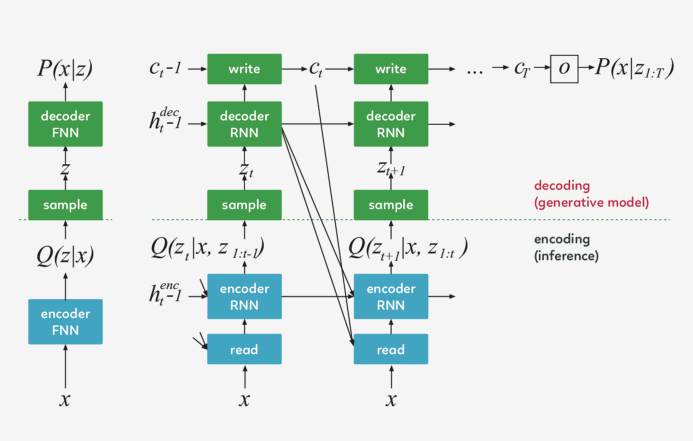
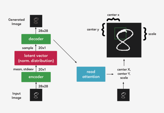
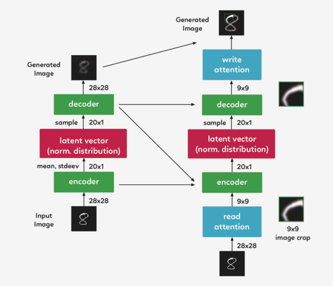
左：傳統(tǒng)變分自動(dòng)編碼器 在生成過程中，從先前的 P（z）中提取一個(gè)樣本 z ，并通過前饋?zhàn)g碼器網(wǎng)絡(luò)來計(jì)算給定樣本的輸入 P（x_z）的概率。 在推理過程中，輸入 x 被傳遞到編碼器網(wǎng)絡(luò)，在潛在變量上產(chǎn)生一個(gè)近似的后驗(yàn) Q(z|x) 。在訓(xùn)練過程中，從 Q(z|x) 中抽取 z，然后用它計(jì)算總描述長(zhǎng)度 KL ( Q (Z|x)∣∣ P(Z)?log(P(x|z))，該長(zhǎng)度隨隨機(jī)梯度的下降（https://en.wikipedia.org/wiki/Stochastic_gradient_descent）而減小至最小值。

右：DRAW網(wǎng)絡(luò) 在每一個(gè)步驟中，都會(huì)將先前 P（z）中的一個(gè)樣本 z_t 傳遞給遞歸解碼器網(wǎng)絡(luò)，該網(wǎng)絡(luò)隨后會(huì)修改 canvas matrix 的一部分。最后一個(gè) canvas matrix cT 用于計(jì)算 P（x|z_1:t）。 在推理過程中，每個(gè) time-step 都會(huì)讀取輸入，并將結(jié)果傳遞給編碼器 RNN，然后從上一 time-step 中的 RNN 指定讀取位置，編碼器 RNN 的輸出用于計(jì)算該 time-step 的潛在變量的近似后驗(yàn)值。 損失函數(shù) 最后一個(gè) canvas matrix cT 用于確定輸入數(shù)據(jù)的模型 D(X | cT)的參數(shù)。如果輸入是二進(jìn)制的，D 的自然選擇呈伯努利分布，means 由σ(cT) 給出。重建損失 Lx 定義為 D 下 x 的負(fù)對(duì)數(shù)概率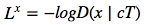：? ? ? ? ? The latent loss 潛在distributions序列??的潛在損失?被定義為源自??

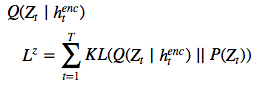
的潛在先驗(yàn) P(Z_t)的簡(jiǎn)要 KL散度。 鑒于這一損失取決于由??繪制的潛在樣本 z_t ，因此其反過來又決定了輸入 x。如果潛在 distribution是一個(gè)?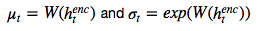這樣的 diagonal Gaussian ，P(Z_t) 便是一個(gè)均值為 0，且具有標(biāo)準(zhǔn)離差的標(biāo)準(zhǔn) Gaussian，這種情況下方程則變?yōu)??

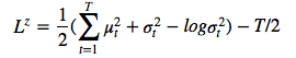
。 網(wǎng)絡(luò)的總損失 L 是重建和潛在損失之和的期望值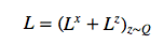：?? ? ? ? 對(duì)于每個(gè)隨機(jī)梯度下降，我們使用單個(gè) z 樣本進(jìn)行優(yōu)化。 ? L^Z 可以解釋為從之前的序列向解碼器傳輸潛在樣本序列 z_1:T 所需的 NAT 數(shù)量，并且（如果 x 是離散的）L^x 是解碼器重建給定 z_1:T 的 x 所需的 NAT 數(shù)量。因此，總損失等于解碼器和之前數(shù)據(jù)的預(yù)期壓縮量。 ? 改善圖片 ? 正如 EricJang 在他的文章中提到的，讓我們的神經(jīng)網(wǎng)絡(luò)僅僅“改善圖像”而不是“一次完成圖像”會(huì)更容易些。正如人類藝術(shù)家在畫布上涂涂畫畫，并從繪畫過程中推斷出要修改什么，以及下一步要繪制什么。 ? 改進(jìn)圖像或逐步細(xì)化只是一次又一次地破壞我們的聯(lián)合 distribution P(C)?，導(dǎo)致潛在變量鏈 C1,C2,…CT?1 呈現(xiàn)新的變量分布 P(CT) 。 ? ? ??

訣竅是多次從迭代細(xì)化分布 P(Ct|Ct?1)中取樣，而不是直接從 P(C) 中取樣。 在 DRAW 模型中，P(Ct|Ct?1) 是所有 t 的同一 distribution，因此我們可以將其表示為以下遞歸關(guān)系（如果不是，那么就是Markov Chain而不是遞歸網(wǎng)絡(luò)了）。

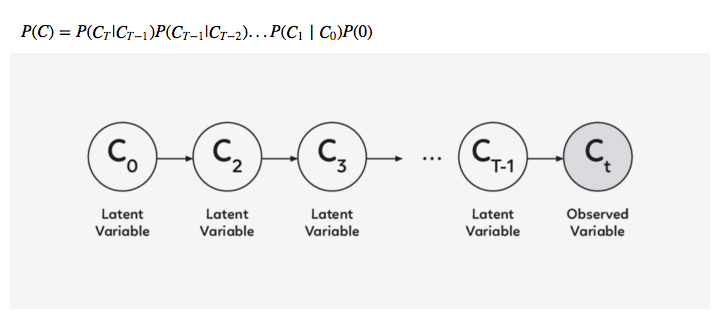
DRAW模型的實(shí)際應(yīng)用 假設(shè)你正在嘗試對(duì)數(shù)字 8 的圖像進(jìn)行編碼。每個(gè)手寫數(shù)字的繪制方式都不同，有的樣本 8 可能看起來寬一些，有的可能長(zhǎng)一些。如果不注意，編碼器將被迫同時(shí)捕獲所有這些小的差異。

但是……如果編碼器可以在每一幀上選擇一小段圖像并一次檢查數(shù)字 8 的每一部分呢？這會(huì)使工作更容易，對(duì)吧？

同樣的邏輯也適用于生成數(shù)字。注意力單元將決定在哪里繪制數(shù)字 8 的下一部分-或任何其他部分-而傳遞的潛在矢量將決定解碼器生成多大的區(qū)域。 基本上，如果我們把變分的自動(dòng)編碼器（VAE）中的潛在代碼看作是表示整個(gè)圖像的矢量，那么繪圖中的潛在代碼就可以看作是表示筆畫的矢量。最后，這些向量的序列實(shí)現(xiàn)了原始圖像的再現(xiàn)。

好吧，那么它是如何工作的呢？

在一個(gè)遞歸的 VAE 模型中，編碼器在每一個(gè) timestep 會(huì)接收整個(gè)輸入圖像。在 Draw 中，我們需要將焦點(diǎn)集中在它們之間的 attention gate 上，因此編碼器只接收到網(wǎng)絡(luò)認(rèn)為在該 timestep 重要的圖像部分。第一個(gè) attention gate 被稱為“Read”attention。 “Read”attention分為兩部分： 選擇圖像的重要部分和裁剪圖像

選擇圖像的重要部分 為了確定圖像的哪一部分最重要，我們需要做些觀察，并根據(jù)這些觀察做出決定。在 DRAW中，我們使用前一個(gè) timestep 的解碼器隱藏狀態(tài)。通過使用一個(gè)簡(jiǎn)單的完全連接的圖層，我們可以將隱藏狀態(tài)映射到三個(gè)決定方形裁剪的參數(shù)：中心 X、中心 Y 和比例。

裁剪圖像 現(xiàn)在，我們不再對(duì)整個(gè)圖像進(jìn)行編碼，而是對(duì)其進(jìn)行裁剪，只對(duì)圖像的一小部分進(jìn)行編碼。然后，這個(gè)編碼通過系統(tǒng)解碼成一個(gè)小補(bǔ)丁。 現(xiàn)在我們到達(dá) attention gate 的第二部分，“write”attention，（與“read”部分的設(shè)置相同），只是“write”attention 使用當(dāng)前的解碼器，而不是前一個(gè) timestep 的解碼器。

雖然可以直觀地將注意力機(jī)制描述為一種裁剪，但實(shí)踐中使用了一種不同的方法。在上面描述的模型結(jié)構(gòu)仍然精確的前提下，使用了gaussian filters矩陣，沒有利用裁剪的方式。我們?cè)贒RAW 中取了一組每個(gè) filter 的中心間距都均勻的gaussian filters 矩陣。 代碼一覽 我們?cè)?Eric Jang 的代碼的基礎(chǔ)上，對(duì)其進(jìn)行一些清理和注釋，以便于理解.

# first we import our librariesimport tensorflow as tffrom tensorflow.examples.tutorials import mnistfrom tensorflow.examples.tutorials.mnist import input_dataimport numpy as npimport scipy.miscimport os Eric 為我們提供了一些偉大的功能，可以幫助我們構(gòu)建 “read” 和 “write” 注意門徑，還有過濾我們將使用的初始狀態(tài)功能，但是首先，我們需要添加新的功能，來使我們能創(chuàng)建一個(gè)密集層并合并圖像。并將它們保存到本地計(jì)算機(jī)中，以獲取更新的代碼。

# fully-conected layerdef dense(x, inputFeatures, outputFeatures, scope=None, with_w=False): with tf.variable_scope(scope or "Linear"): matrix = tf.get_variable("Matrix", [inputFeatures, outputFeatures], tf.float32, tf.random_normal_initializer(stddev=0.02)) bias = tf.get_variable("bias", [outputFeatures], initializer=tf.constant_initializer(0.0)) if with_w: return tf.matmul(x, matrix) + bias, matrix, bias else: return tf.matmul(x, matrix) + bias # merge imagesdef merge(images, size): h, w = images.shape[1], images.shape[2] img = np.zeros((h * size[0], w * size[1])) for idx, image in enumerate(images): i = idx % size[1] j = idx / size[1] img[j*h:j*h+h, i*w:i*w+w] = image return img # save image on local machine def ims(name, img): # print img[:10][:10]scipy.misc.toimage(img,cmin=0,cmax=1).save(name) 現(xiàn)在讓我們把代碼放在一起以便完成。

# DRAW implementationclass draw_model(): def __init__(self): # First we download the MNIST dataset into our local machine. self.mnist = input_data.read_data_sets("data/", one_hot=True) print "------------------------------------" print "MNIST Dataset Succesufully Imported" print "------------------------------------" self.n_samples = self.mnist.train.num_examples # We set up the model parameters # ------------------------------ # image width,height self.img_size = 28 # read glimpse grid width/height self.attention_n = 5 # number of hidden units / output size in LSTM self.n_hidden = 256 # QSampler output size self.n_z = 10 # MNIST generation sequence length self.sequence_length = 10 # training minibatch size self.batch_size = 64 # workaround for variable_scope(reuse=True) self.share_parameters = False # Build our model self.images = tf.placeholder(tf.float32, [None, 784]) # input (batch_size * img_size) self.e = tf.random_normal((self.batch_size, self.n_z), mean=0, stddev=1) # Qsampler noise self.lstm_enc = tf.nn.rnn_cell.LSTMCell(self.n_hidden, state_is_tuple=True) # encoder Op self.lstm_dec = tf.nn.rnn_cell.LSTMCell(self.n_hidden, state_is_tuple=True) # decoder Op # Define our state variables self.cs = [0] * self.sequence_length # sequence of canvases self.mu, self.logsigma, self.sigma = [0] * self.sequence_length, [0] * self.sequence_length, [0] * self.sequence_length # Initial states h_dec_prev = tf.zeros((self.batch_size, self.n_hidden)) enc_state = self.lstm_enc.zero_state(self.batch_size, tf.float32) dec_state = self.lstm_dec.zero_state(self.batch_size, tf.float32) # Construct the unrolled computational graph x = self.images for t in range(self.sequence_length): # error image + original image c_prev = tf.zeros((self.batch_size, self.img_size**2)) if t == 0 else self.cs[t-1] x_hat = x - tf.sigmoid(c_prev) # read the image r = self.read_basic(x,x_hat,h_dec_prev) #sanity check print r.get_shape() # encode to guass distribution self.mu[t], self.logsigma[t], self.sigma[t], enc_state = self.encode(enc_state, tf.concat(1, [r, h_dec_prev])) # sample from the distribution to get z z = self.sampleQ(self.mu[t],self.sigma[t]) #sanity check print z.get_shape() # retrieve the hidden layer of RNN h_dec, dec_state = self.decode_layer(dec_state, z) #sanity check print h_dec.get_shape() # map from hidden layer self.cs[t] = c_prev + self.write_basic(h_dec) h_dec_prev = h_dec self.share_parameters = True # from now on, share variables # Loss function self.generated_images = tf.nn.sigmoid(self.cs[-1]) self.generation_loss = tf.reduce_mean(-tf.reduce_sum(self.images * tf.log(1e-10 + self.generated_images) + (1-self.images) * tf.log(1e-10 + 1 - self.generated_images),1)) kl_terms = [0]*self.sequence_length for t in xrange(self.sequence_length): mu2 = tf.square(self.mu[t]) sigma2 = tf.square(self.sigma[t]) logsigma = self.logsigma[t] kl_terms[t] = 0.5 * tf.reduce_sum(mu2 + sigma2 - 2*logsigma, 1) - self.sequence_length*0.5 # each kl term is (1xminibatch) self.latent_loss = tf.reduce_mean(tf.add_n(kl_terms)) self.cost = self.generation_loss + self.latent_loss # Optimization optimizer = tf.train.AdamOptimizer(1e-3, beta1=0.5) grads = optimizer.compute_gradients(self.cost) for i,(g,v) in enumerate(grads): if g is not None: grads[i] = (tf.clip_by_norm(g,5),v) self.train_op = optimizer.apply_gradients(grads) self.sess = tf.Session() self.sess.run(tf.initialize_all_variables()) # Our training function def train(self): for i in xrange(20000): xtrain, _ = self.mnist.train.next_batch(self.batch_size) cs, gen_loss, lat_loss, _ = self.sess.run([self.cs, self.generation_loss, self.latent_loss, self.train_op], feed_dict={self.images: xtrain}) print "iter %d genloss %f latloss %f" % (i, gen_loss, lat_loss) if i % 500 == 0: cs = 1.0/(1.0+np.exp(-np.array(cs))) # x_recons=sigmoid(canvas) for cs_iter in xrange(10): results = cs[cs_iter] results_square = np.reshape(results, [-1, 28, 28]) print results_square.shape ims("results/"+str(i)+"-step-"+str(cs_iter)+".jpg",merge(results_square,[8,8])) # Eric Jang's main functions # -------------------------- # locate where to put attention filters on hidden layers def attn_window(self, scope, h_dec): with tf.variable_scope(scope, reuse=self.share_parameters): parameters = dense(h_dec, self.n_hidden, 5) # center of 2d gaussian on a scale of -1 to 1 gx_, gy_, log_sigma2, log_delta, log_gamma = tf.split(1,5,parameters) # move gx/gy to be a scale of -imgsize to +imgsize gx = (self.img_size+1)/2 * (gx_ + 1) gy = (self.img_size+1)/2 * (gy_ + 1) sigma2 = tf.exp(log_sigma2) # distance between patches delta = (self.img_size - 1) / ((self.attention_n-1) * tf.exp(log_delta)) # returns [Fx, Fy, gamma] return self.filterbank(gx,gy,sigma2,delta) + (tf.exp(log_gamma),) # Construct patches of gaussian filters def filterbank(self, gx, gy, sigma2, delta): # 1 x N, look like [[0,1,2,3,4]] grid_i = tf.reshape(tf.cast(tf.range(self.attention_n), tf.float32),[1, -1]) # individual patches centers mu_x = gx + (grid_i - self.attention_n/2 - 0.5) * delta mu_y = gy + (grid_i - self.attention_n/2 - 0.5) * delta mu_x = tf.reshape(mu_x, [-1, self.attention_n, 1]) mu_y = tf.reshape(mu_y, [-1, self.attention_n, 1]) # 1 x 1 x imgsize, looks like [[[0,1,2,3,4,...,27]]] im = tf.reshape(tf.cast(tf.range(self.img_size), tf.float32), [1, 1, -1]) # list of gaussian curves for x and y sigma2 = tf.reshape(sigma2, [-1, 1, 1]) Fx = tf.exp(-tf.square((im - mu_x) / (2*sigma2))) Fy = tf.exp(-tf.square((im - mu_x) / (2*sigma2))) # normalize area-under-curve Fx = Fx / tf.maximum(tf.reduce_sum(Fx,2,keep_dims=True),1e-8) Fy = Fy / tf.maximum(tf.reduce_sum(Fy,2,keep_dims=True),1e-8) return Fx, Fy # read operation without attention def read_basic(self, x, x_hat, h_dec_prev): return tf.concat(1,[x,x_hat]) # read operation with attention def read_attention(self, x, x_hat, h_dec_prev): Fx, Fy, gamma = self.attn_window("read", h_dec_prev) # apply parameters for patch of gaussian filters def filter_img(img, Fx, Fy, gamma): Fxt = tf.transpose(Fx, perm=[0,2,1]) img = tf.reshape(img, [-1, self.img_size, self.img_size]) # apply the gaussian patches glimpse = tf.batch_matmul(Fy, tf.batch_matmul(img, Fxt)) glimpse = tf.reshape(glimpse, [-1, self.attention_n**2]) # scale using the gamma parameter return glimpse * tf.reshape(gamma, [-1, 1]) x = filter_img(x, Fx, Fy, gamma) x_hat = filter_img(x_hat, Fx, Fy, gamma) return tf.concat(1, [x, x_hat]) # encoder function for attention patch def encode(self, prev_state, image): # update the RNN with our image with tf.variable_scope("encoder",reuse=self.share_parameters): hidden_layer, next_state = self.lstm_enc(image, prev_state) # map the RNN hidden state to latent variables with tf.variable_scope("mu", reuse=self.share_parameters): mu = dense(hidden_layer, self.n_hidden, self.n_z) with tf.variable_scope("sigma", reuse=self.share_parameters): logsigma = dense(hidden_layer, self.n_hidden, self.n_z) sigma = tf.exp(logsigma) return mu, logsigma, sigma, next_state def sampleQ(self, mu, sigma): return mu + sigma*self.e # decoder function def decode_layer(self, prev_state, latent): # update decoder RNN using our latent variable with tf.variable_scope("decoder", reuse=self.share_parameters): hidden_layer, next_state = self.lstm_dec(latent, prev_state) return hidden_layer, next_state # write operation without attention def write_basic(self, hidden_layer): # map RNN hidden state to image with tf.variable_scope("write", reuse=self.share_parameters): decoded_image_portion = dense(hidden_layer, self.n_hidden, self.img_size**2) return decoded_image_portion # write operation with attention def write_attention(self, hidden_layer): with tf.variable_scope("writeW", reuse=self.share_parameters): w = dense(hidden_layer, self.n_hidden, self.attention_n**2) w = tf.reshape(w, [self.batch_size, self.attention_n, self.attention_n]) Fx, Fy, gamma = self.attn_window("write", hidden_layer) Fyt = tf.transpose(Fy, perm=[0,2,1]) wr = tf.batch_matmul(Fyt, tf.batch_matmul(w, Fx)) wr = tf.reshape(wr, [self.batch_size, self.img_size**2]) return wr * tf.reshape(1.0/gamma, [-1, 1]) model = draw_mod