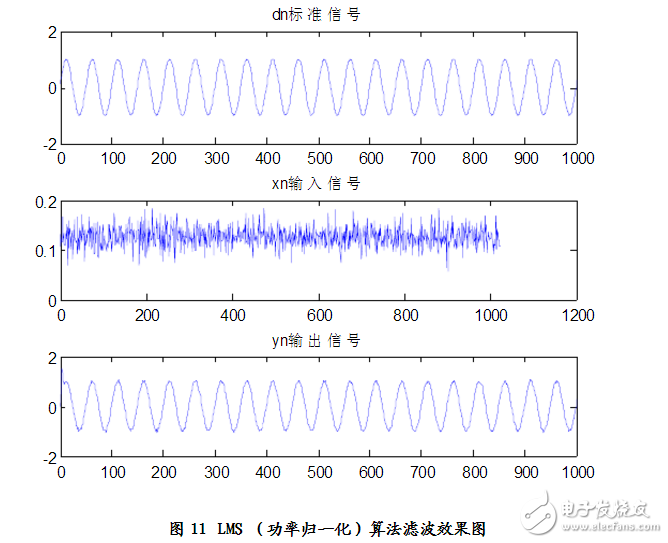
方案3——功率歸一化LMS算法的實現

　　功率歸一化，與歸一化算法一樣，也只是在對u（k）的取值方面有一定的差別。功率歸一化中定義u（k）=a/g2x（k），其中g2x表示x（k）的方差。由a/g2x（k）=dg2x（k-1）+e2（k）可知，d《（0，1），0《a《2/m，其中M為濾波器的階數。同時也為了方便起見，我們暫且定義a=1/M，d=0.5。

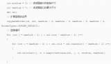
　　功率歸一化LMS算法編程為：

　　for n=2:M

　　xn=sin（4*pi*n/100）+vn;

　　yn（n）=w1（n）*xn（n）+w2（n）*xn（n-1）;

　　e（n）=xn（n）-yn（n）;

　　gx2（n）=d*gx2（n-1）+e（n）*e（n）; u（n）=a/（gx2（n））;

　　w1（n+1）=w1（n）+2*u（n）*e（n）*xn（n）;

　　w2（n+1）=w2（n）+2*u（n）*e（n）*xn（n-1）;

　　end

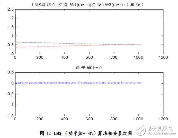
　　仿真結果：見圖11、圖12

　　分析得：n=8

　　Elapsed time is 0.078000 seconds.

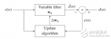
　　LMS（least mean square）自適應濾波算法matlab實現

　　以下是matlab幫助文檔中lms示例程序，應用在一個系統辨識的例子上。整個濾波的過程就兩行，用紅色標識。

　　x = randn（1，500）; % Input to the filter

　　b = fir1（31，0.5）; % FIR system to be identified

　　n = 0.1*randn（1，500）; % Observation noise signal

　　d = filter（b，1，x）+n; % Desired signal

　　mu = 0.008; % LMS step size.

　　ha = adaptfilt.lms（32，mu）;

　　［y，e］ = filter（ha，x，d）;

　　subplot（2，1，1）; plot（1:500，［d;y;e］）;

　　title（‘System Identification of an FIR Filter’）;

　　legend（‘Desired’，‘Output’，‘Error’）;

　　xlabel（‘Time Index’）; ylabel（‘Signal Value’）;

　　subplot（2，1，2）; stem（［b.‘，ha.coefficients.’］）;

　　legend（‘Actual’，‘Estimated’）;

　　xlabel（‘Coefficient #’）; ylabel（‘Coefficient Value’）;

　　grid on;

　　這實在看不出什么名堂，就學習目的而言，遠不如自己寫一個出來。整個濾波的過程用紅色標識。

　　%% System Identification （SID）

　　% This demonstration illustrates the application of LMS adaptive filters to

　　% system identification （SID）。

　　%

　　% Author（s）： X. Gumdy

　　% Copyright 2008 The Funtech， Inc.

　　%% 信號產生

　　clear all;

　　N = 1000 ;

　　x = 10 * randn（N，1）; % 輸入信號

　　b = fir1（31，0.5）; % 待辨識系d

　　n = randn（N，1）;

　　d = filter（b，1，x）+n; % 待辨識系統的加噪聲輸出

　　%% LMS 算法手工實現

　　sysorder = 32;

　　maxmu = 1 / （x‘*x / N * sysorder）;% 通過估計tr（R）來計算mu的最大值

　　mu = maxmu / 10;

　　w = zeros （ sysorder ， 1 ） ;

　　for n = sysorder ： N

　　u = x（n-sysorder+1:n） ;

　　y（n）= w’ * u;

　　e（n） = d（n） - y（n） ;

　　w = w + mu * u * e（n） ;

　　end

　　y = y‘;

　　e = e’;

　　%% 畫圖

　　figure（1）;

　　subplot（2，1，1）; plot（（1:N）‘，［d，y，e］）;

　　title（’System Identification of an FIR Filter‘）;

　　legend（’Desired‘，’Output‘，’Error‘）;

　　xlabel（’Time Index‘）; ylabel（’Signal Value‘）;

　　subplot（2，1，2）; stem（［b’， w］）;

　　legend（‘Actual’，‘Estimated’）;

　　xlabel（‘Coefficient #’）; ylabel（‘Coefficient Value’）;

　　grid on;